The Measurement of Shear by the Distortion of Spheres

Boxes are point functions, that is, they are defined at a point in the matrix, which means that they express the distortion that occurs at that point in the strained medium. In some situations, it is informative to obtain an impression of what is occurring to an array of points that surround a particular point in the medium. To visualize the strain, we create a bubble about the test location and watch how that bubble is distorted as the medium is strained.

Ideally, we would like to have a sphere of points surrounding the test location, but for calculation it is necessary to select a set of points in the surface of a sphere. How we select those points can determine how true the calculation is to the ideal. In particular, it is important that the selected point be equally distributed in the surface of the hypothetical bubble. Using equally spaced point in a longitude/latitude type grid will not yield a symmetrical data set, since the gridlines will tend to converge at the poles.

First, we will create a set of equally spaced points, actually two interdigitated sets of equally spaced points, by computing the vertices of two platonic solids. The data sets can be distorted by strain in the medium that they occupy, giving an image of the distortions. Then, using the insights provided by those calculations, we will perform some algebraic calculations to examine the analytic form of the distortions. Those analytic findings will lead us to a consideration of the similarity of the compression/expansion strain and shear strain.

Calculating a data set of equally spaced points on a sphere

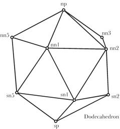
If we consider an imaginary sphere embedded in the matrix that is distorted by the strains in the material, then we can visualize the strain by examining the distortion of the sphere. In lieu of a sphere, for computational purposes, we will use an equally spaced array of points in the surface of the sphere. To that end, we need to compute a set of points that are evenly distributed over the surface of a unit sphere. Such a set of points can be obtained by using the vertices of a regular polyhedron inscribed within the sphere, such as a dodecahedron, which has 12 vertices separated by equilateral triangles.

The twelve vertices include a north pole (np) and a south pole (sp) and two sets of 5 vertices in the northern and southern mid-latitudes (nn₁ -> nn₅ and sn₁ -> sn₅). These vertices are approximately 63.435° away from the polar nodes, which is the angular excursion subtended by one side of an equilateral triangle that forms a face of the dodecahedron. The northern nodes are offset a tenth of a circle (36°) relative to the southern nodes. Of course, the designation of which points are the poles and which are nodes is arbitrary, but by assuming this configuration one can compute the values of the points that lie at the vertices. Once one has a set of points they can be rotated about any axis of rotation to obtain any configuration desired for the purposes of calculation.

The calculation starts with the assumption that the north pole node is at +k and the south pole node at –k (). Then, the north pole vector is rotated 63.435° about an axis of rotation equal to j, to obtain the first northern node

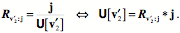
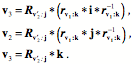
That vector is rotated about +k through 4 successive 72° rotations to obtain the remaining northern nodes

The south pole vector is rotated about the – j axis, through 63.435°, and then 36° about the +k axis to obtain the first southern node.

Once again, the first southern node is rotated through 4 successive rotations of 72° about the +k axis to obtain the remaining southern nodes.

The set of 12 equally spaced points on a unit sphere is as follows:

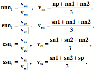
A set of 20 equally spaced points can be obtained using the centers of the faces of the dodecahedron, which are the vertices of an icosahedron. There are four sets of five points, with each point in a set advanced 72° around the pole from the last.

If the first node in the northernmost tier is nnn₁, then it is the unit vector in the direction of the average of the three dodecahedral vertices np, nn1, and nn2. The first node in the tier north of the equator (enn₁) will be the unit vector in the direction of the average of nn1, nn2, and sn1. The first node in the tier south of the equator (esn₁) will be the unit vector in the direction of the average of sn1, sn2, and nn2. Finally, the first node in the tier in the southernmost tier (ssn₁) will be the unit vector in the direction of the average of sp, sn1, and sn2.

For each tier the remaining four vertices are obtained by rotation the first vertex through 72° of angular excursion about the north pole axis.

The values are as follows.

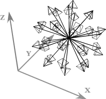
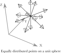
These two sets of equally spaced points can be combined to obtain a denser covering of the sphere. The 32 point data set is good for calculations in that they provide a dense enough coverage to make computed values good approximations to the values for a sphere, but for illustration we will use the 12 vertices of an inscribed dodecahedron. It is easier to appreciate the distortions due to the strains.

The set of 32 points that lie at the vertices of an inscribed icosahedron and an inscribed dodecahedron where the vertices of one lie in the centers of the faces for the other. There are 20 vectors to the vertices of the icosahedron and 12 vectors to the vertices of the dodecahedron.

By using this data set it is possible to experiment with the different types of strain using a test object that is symmetrical and not strongly oriented to any particular directions. The experiments suggest how one might attack the problem of describing strain in more analytical terms.

Strain and Distortions of an Embedded Sphere

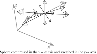
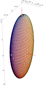
For experimental purposes, we start with a set of equally spaced points on the surface of a unit sphere. The unstrained points for a set of 12 equally spaced points are illustrated above.

We can set the axes of the strain to lie in any direction. The strain axes may be the directions of compression or expansion or they may define the directions of the axes that are sheared. To compute the strain for the sphere, each of the vectors in the array is projected upon the three unstrained axes of strain, then the transformation due to the strain is computed for each component, and finally the components are recombined to obtain the strained vector. This calculation was described in the last chapter,

Compression and Expansion

If the sphere is compressed by half along an axis in the direction of y = -x and stretched two-fold along an axis is the direction of y = x, then its vectors will appear as in the above figure. The axes of strain for this example are in the directions y = x, y = -x, and z. That is, the axes of strain are the basis frame rotated +45° about the z vector. The vectors that were more aligned with the y = x direction are stretched and the vectors more aligned with the y = -x direction are compressed. The vertical component of each vector is unchanged. It is apparent that the sphere now resembles a prolate ellipsoid with the long axis in the direction of y = x. If the sphere were compressed in one direction and allowed to expand in the perpendicular plane, then the strained sphere would appear to be an oblate ellipsoid.

Shear Strain

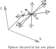
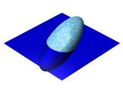
If we leave the strain axes in the same orientation, that is, rotated 45° about the vertical axis, and cause the strain to be a tilt of the vertical strain axis 45° towards the first horizontal axis, then the sphere is sheared so that it will look like the above illustration. The strained sphere is again a prolate ellipsoid, but with the long axis tilted up at approximately a 45° angle in the direction of y = x.

With this model, it is possible to explore a great many situations in which we vary the types, magnitudes, and directions of the strains. We can also combine strains and see how they interact. The little that has been demonstrated here is suggestive of directions that may be profitably pursued with more analytical methods.

Analytical Calculations

The advantage of the model using equally spaced points on a unit sphere is that we can choose any configuration and obtain the results with equal ease. So one can try a wide variety of situations to obtain an intuitive feel for the nature of the strain distortions and one can rotate the computed image in the computer to see how the points appear from any vantage point. The disadvantage is that it is difficult to obtain quantitative information from the image. The image may always be analyzed by calculations on its data set, but the results are always approximations. It is also useful to use analytical methods to obtain exact results. However, it is easier to use such methods if we simplify the situation being analyzed. Having developed our intuitions for the full spectrum of possible situations with the model, it is easier to see where simplification is possible without simplifying away the properties that we wish to study.

Compression and expansion produce an ellipsoidal distortion

Calculations, using the larger data set indicate that the strained spheres in both cases are probably ellipsoids. We can check that observation by considering a simpler problem, one more amenable to algebraic analysis. Consider a section of a sphere, which is a circle.

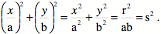
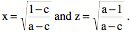
Let the strains be compression and/or extension in the plane of the circle. So, the value of x is divided by ‘a’ and the value of y is divided by ‘b’.

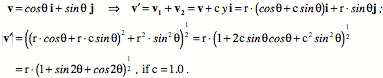
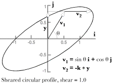
However, that is the formula for an ellipse. Consequently, the cross-section of the strained sphere is an ellipse in all three orthogonal planes defined by the axes of strain, and the surface is an ellipsoid.

Shear produces a rotated ellipsoidal distortion

Consider a similar calculation for shear strain. Take a circular cross-section of the sphere with a radius of ‘r’, in the plane of the shear. We add a vector component in the direction of the shear that is proportional to the magnitude of the y component.

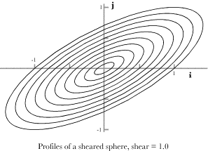
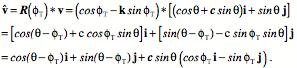
The derivative of the vector length with respect to angle (q) has minima and maxima at four angles, . If we plot the expression for the profile, then it is apparent which is a maxima and which a minima. The maxima and minima are not a function of the radius.

The circular profile is tilted into an elliptical shape that is inclined at an angle to the positive i axis. It would appear that the effect of the shear strain is to make the sphere have an ellipsoidal shape. When we compute the changes for a series of circular profiles in the plane of the shear, all the profiles have the same amount of tilt.

The amount of tilt is the arccosine of the scalar of the ratio of a unit vector in the direction of the maxima to a unit vector aligned with the i axis.

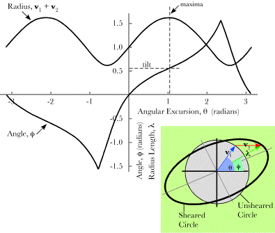
When we plug in the angle that gives the maximal point on the sheared profile (58.28°) the tilt of the long axis of the ellipse is at an angle of 31.72° to the i axis.

The angular excursion at the maximal point (q) and the tilt (f)

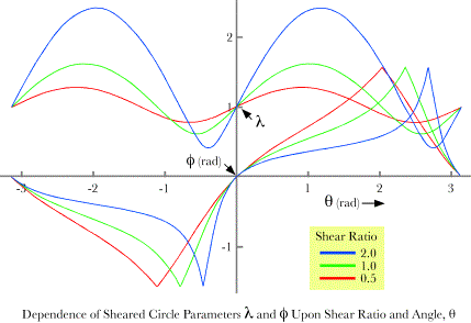
There are two angles of interest in understanding the orientation of the sheared sphere. The first is the value of the angular excursion at the maximal deviation from a circle, q, and the other is the tilt of the sheared circle, f. The maximal deviation is the sum of a radius of the original unsheared circle, , and the horizontal shear parallel with the i axis, . The angle q is the angle that forms with the horizontal axis. The angle f is the angle between the i axis and the sum of the two vectors, l.

In the above figure the length of the sum of the two component vectors, l, is computed for all values of q. Similarly, the angle to the sum of the component vectors, f, has been computed for all values of q. In this instance f is the angle between the horizontal axis and l. If we draw a vertical line through the maximum in the plot of the length of l, then it will intersect the value of the plot of f that is equal to the tilt of the sheared circle.

As the magnitude of the shear increases, the excursion of the upper curve grows greater and the minimal parts of the curve more angular. The curve for f becomes more non-linear and the tilt at the maxima is smaller. For small amounts of shear the curves for f approach a saw-tooth shape and the curve for l becomes more sinusoidal. For large shear ratios the curve for f is nearly flat and nearly equal to zero radians, except for the minima of l, when it rapidly goes to p/2. The curves for l become approximately a series of positive sinusoidal peaks.

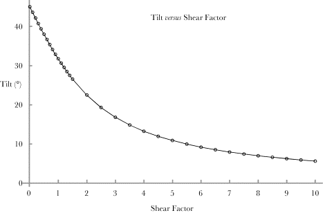
For three shear ratios, the curves for l and f as functions of the angle q are plotted upon a common set of axes. The radial distance from the origin to the sheared circle, l, is calculated for all angles about the origin, q. The maximal value for l is occurs for the longest axis of the sheared circle and the minimal value occurs for the shortest axis. The value of f when l is maximal is the tilt of the sheared circle.

As the shear ratio increases the maxima for l shifts to greater values, until it reaches p/2 for very large shear factors. The minima for l is always separated from the maxima by 90° (p/2 radians). As the shear ratio increases, the value of f at the maxima decreases to approach 0° (0.0 radians).

Is the tilt of the ellipse linearly proportional to the shear?

The question naturally arises of how the amount of tilt depends upon the amount of shear. If one systematically computes the amount of tilt for the ellipsoid relative to the i axis as a function of the amount of shear, the relationship turns out to be curvilinear. For small amounts of shear (<1.0) the relationship is nearly linear. For large amounts of shear, the curve becomes asymptotic to the tilt = 0° line.

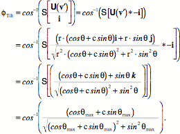
This relationship makes sense because the sheared circle is moderately distorted from a circle for small amounts of shear and the distortion is greatest for angles of about 45°, where the vector for the circle is the dominant vector in the vector sum. As the shear becomes proportionately greater it becomes the dominant vector and it is greatest when the angle is close to 90°, but the ellipse becomes flatter, because the shear is much greater than the radius of the circle and the sheared circle is stretched in the direction of the i axis.

Are the shear ellipsoids actually elliptical?

It was assumed the profiles that were calculated were ellipses, but their shape should be established precisely. Perhaps the simplest way to do so is to rotate the profile so that its long axis is aligned with the i axis, which will simplify its description and make it more symmetrical. It has been established that the tilt of the profile is a definite angle, which we will symbolize with the letter . Then the rotation that turns the profile into alignment with the i and j axes is written as follows.

The first two terms are the description of a unit circle and the last term is a vector with a constant direction and a length that varies sinusoidally with the angular excursion from the i axis, q. It is not obvious that that combination describes an ellipse, but plotting the components gives an ellipse. That is largely due to the phase differences between the terms that describe a unit circle and the terms that describe the variable length vector.

The equivalency between a shear ellipsoid and a compressive-tensile ellipsoid

It is interesting that both compression/expansion and shear give a distortion that is an ellipsoid. This means that though they are different processes there is a formal equivalency between the two. It is not a full equivalency because sheared spheres are always prolate ellipsoids, that is, flattened cigar shaped. Compressive-tensile strain may lead to prolate or oblate ellipsoids and even to larger or smaller spheres. Consequently, it is more accurate to say that compressive-tensile strain may produce the same distortion as a shear strain. However, they are not equivalent in that the force that could produce the equivalent compressive distortion is a fictitious force. It is also a force that constantly changes direction to match a shear force that only changes in magnitude. As the shear ratio increases, the sheared sphere becomes more elongated and its tilt with respect to the shear plane becomes smaller. The equivalent compressive strain is perpendicular to the long axis of the ellipsoid, therefore, as the tilt decreases, the direction of the compression is more and more perpendicular to the shear plane. In addition, for situations when the two ellipsoids are equivalent, the compression/expansion is constrained to be constant volume and expansion is allowed in only one direction, along the long axis of the ellipsoid.

Even though the equivalence is not realistic, the formal equivalence between a sheared sphere and a particular compressive/expansive strain can be used to derive some properties of a sheared sphere. If one knows the orientation of the axes of the strained sphere, then the compression-expansive strain that would have produced it are aligned with those axes. The strain array will be aligned with the axes of the ellipsoid. This observation may be used to determine the strain that leads to the observed ellipsoid. We first compute the strain array and rotate it into a canonical orientation. In that orientation, it is easy to compute the plane of the shear and the direction of the sheared vector.

Derivation of the shear plane

Let the longest axis of the ellipsoid be. There are two perpendicular axes, and . Let the next longest be and the shortest be . If we know the vector for then we can compute the rotation that will rotate it into one of the coordinate axes, say k.

We can then collapse all the points of the sheared sphere into the i, j – plane and determine the next longest axis, . That axis can be rotated into another coordinate axis, say the j axis.

The rotation quaternion has a vector component that is a multiple of k.

The last axis, , is the ratio of the transformed first axis to the transformed second axis, which is in the direction of i. The coordinate axes transform as follows.

Consequently, we can rotate the shear ellipsoid into alignment with the coordinate axes, work out relationships for the canonical ellipsoid aligned with the coordinate axes, and then rotate the result back into alignment with the actual ellipsoid.

Once we have obtained the canonical ellipsoid for the equivalent compressive-tensile strain, it is possible to compute the shear plane and sheared axis for the shear ellipsoid. If the strain is due to shear, then there should be a section through the ellipsoid that is circular, which is aligned with the plane of the shear, because the shear is zero in that plane. A perpendicular to that plane will be the sheared axis.

In a shear ellipsoid that has experienced a pure shear, the volume of the ellipsoid remains unity and there is one axis that is unchanged by the strain (), one that is elongated (), and one that is shortened (). The canonical ellipsoid may be expressed as follows.

The length of the axis is unity and it lies in the shear plane of the sphere. We need to find a second vector in the shear plane in order to define it. The orthogonal vector will extend from the center of the ellipsoid to a point in the midline section of the ellipsoid in the i,k-plane (). The formula for that ellipse in that plane is as follows.

The distance to the point is unity.

Therefore,

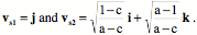
The vectors that define the shear plane in the canonical orientation are –

The length of both vectors is 1.0 and the angle between them is a right angle. The sheared axis is the ratio of the two vectors.

The ellipsoid for the radii looks like the following figure. The white dots sketch the circular section of its surface. If you plug in the values for ‘a’ and ‘c’, the vectors that define the plane are

The intersecting plane is tilted 54.736° up about the j axis. Of course, the plane with the negative of the i component is equally valid and it is the one illustrated above. The plane that intersects the ellipsoid is the plane of the shear that will produce the ellipsoid. If we rotate the intersecting plane so that it is horizontal, then that can be more readily seen. The mottled ellipsoid is the strained sphere and the blue plane is the plane of shear at the level with no shear.

To obtain the actual plane of shear it is necessary to reverse the two rotations that moved the shear ellipsoid into the canonical position. Given the three axes of a sheared sphere, one can determine the plane of the shear and the tilt of the ellipsoid, therefore the magnitude of the shear and the direction of the shear. With a bit more trouble, it is possible to determine the shear parameters for combinations of shear and compression.