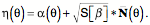
On Evolutes and Frames of Curves

A line is not orientable at points along its length in the usual sense of orientable, but it is possible to attach a frame to a line and obtain useful information about it. Suppose we have a line that is extended in three-dimensional space. The direction of the line at a point along the line is the derivative of the line.

We can define a vector normal to the line at , , where is the limit of the ratio of directions of the line as the interval between the test points approaches zero, the ratio of its tangents.

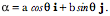
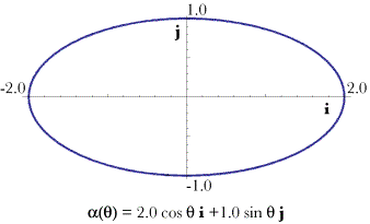
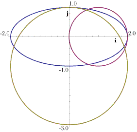
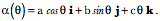
The vector is the vector of a quaternion that defines the curvature of the line at the point . Let that vector be symbolized as , where is bolded, but not italicized.

An example, ellipses:

An ellipse in the i,j-plane, centered upon the origin, is described by the following vector expression.

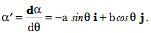
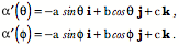
It follows that the tangent to the ellipse is the first derivative of the expression.

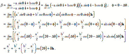
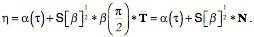
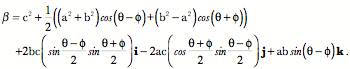
Consequently, the limiting ratio of the tangent vectors, which will be called the turning quaternion, is given by the following expression in which we insert the appropriate expressions in the definition.

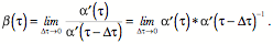
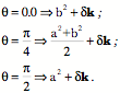
Let the vector of the turning quaternion be , the turning vector. The term is meant to indicate a very small vector component in the direction of k. If the two sampled points are identical, then there is no difference between the tangents and therefore the ratio of the tangents is a scalar. However, given any two non-coincident points on the ellipse there will be a vector in the direction of k. The ratio of tangents is a scalar plus an infinitesimal vector. It is important that the vector component of the quaternion remain non-zero because the unit vector of the quaternion is legitimately k. In this particular example the vector of the quaternion is always the same, because the curve lies in a plane, therefore all tangents to the curve must lie in that plane.

If we insert some instances of points on the ellipse then we can see how behaves.

If the ellipse is a circle, then the expression for reduces to a constant.

It follows from this observation that the magnitude of the scalar component of the quaternion is the square of the radius of the circle that would be tangent to the curve at that point. Consequently, the point in the ellipse where it crosses the i axis has a curvature comparable to a circle with a radius of ‘b’ and the point where it crosses the j axis has a curvature comparable to a circle with a radius of ‘a’.

The ellipse is plotted with the osculating circles at the points {2,0} and {0,1}.

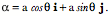
The reasonableness of this is demonstrated in the above figure in which the same ellipse, with axes 2.0 and 1.0, is plotted with circles of those radii touching the ellipse at the appropriate locations. Clearly the circles approximate the ellipse at the points where they touch. The turning quaternion, , gives the osculating circle for each point on the ellipse and, in general, it will give the osculating circle for each point on any curve. An osculating circle is one that ‘kisses’ the curve at a point on the curve.

If one knows the unit tangent to the curve at a point in the curve and the turning quaternion, then it should be possible to compute the center of the circle that osculates the curve at that point, . It lies on the normal to the tangent and the turning vector, a distance equal to the square root of the scalar of the quaternion from the point.

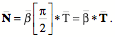
Let the unit vector in the direction of be . For instance, in the example that we have been considering,. The normal to the tangent vector may be obtained by rotating the unit tangent vector 90° about the unit vector of the quaternion.

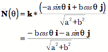
If we apply this expression to the example, we obtain an expression for the normal vector at each point on the ellipse.

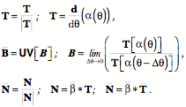
Let us define three mutually orthogonal unit vectors at each point on a curve. They are like the three that we have already seen, except for being unit vectors.

From the last line one can also express the unit vector for the ratio of the tangents, , as the ratio of the unit normal vector to the unit tangent vector.

Now it is possible to write down the center of curvature for a point on a curve. It is the point on the normal to the curve that is a distance equal to the square root of the scalar of from the point on the curve.

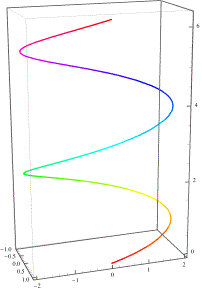
The curve is the evolute of the curve .

A second example, helices:

We can now move to curves in three-dimensional space. The example that will examined is the helix, a curve that moves in an elliptical path as it moves steadily in the perpendicular direction. It is described by the following vector curve.

The tangent vectors for and are readily calculated.

The ratio of the two tangent vectors is straightforward to express, but does require a bit of juggling of trigonometric identities to obtain a convenient form for present purposes.

A helix that traces an ellipse that has a minor axis of 1.0 and a major axis of 2.0 as it ascends at a rate of 0.5 through two cycles.

When the helix traces an ellipse, the tuning quaternion, , varies in both its scalar and vector parts as the angle, , changes. The following table is computed for the illustrated helix, which traces out an ellipse that has a minor axis and a major axis as it ascends steadily in the k direction at a rate of . The square root of the scalar is the , which is the distance to the center of curvature. The i, j, and k columns are the values of those components of the unit vector in the direction of the turning quaternion’s vector.

From the first example, we expect the scalar of the turning quaternion to be greater for than for . Note that the ’s for the major and minor axes are not the same as they were for the ellipse with the same axes. They are larger because of the additional flattening due to the vertical excursion of the curve (2.06 versus 2.0 and 1.12 versus 1.0).

The Components of the Turning Quaternion.

Helix(1.0, 2.0, 0.5}

The helix for which {a, b, c}={1.0, 2.0, 1.0} has been sampled at 10° intervals and the frames computed for the first cycle. The blue arrows are the tangent vectors, the red arrows are the vectors of the turning quaternions, and the green arrows are the normal vectors. All the vectors are the unit vectors.

It is difficult to ‘see’ the frame from tabular data, therefore the above figure shows the frame for 10° intervals along the helix {a, b, c}={1.0, 2.0, 1.0}. The blue vectors are the tangents, which naturally point in the direction of the curve. Actually, the blue vectors are unit vectors in the direction of the tangent vectors, the length of the tangent vectors changes with location, because the projection of the helix into the horizontal plane is an ellipse.

The red vectors are the unit vectors of the turning quaternions, computed from the ratio of the tangent vector 0.001° after the point to the tangent vector 0.001° before the point. Because the slope of the helix as it ascends varies with location, the tilt of the turning vectors also changes. That is readily appreciated by examining the k component of the turning quaternion. The vector of the quaternion shifts with respect to the vertical. If we take the ratio of the unit vector of the turning quaternion to the vertical unit vector, then the cosine of the angle between them is the scalar of the ratio. The angle varies from 14.04° () to 26.56° (). If the helix, H{a,b,c}, has , then the angle is 26.56° at all , and if it has , then the angle is 14.04°. For a helix that has unity for all three values, the angle for all is 45°. Naturally, when, that is when the helix is an ellipse, the angle is 0° and all the turning vectors are perpendicular to the plane of the ellipse. In brief, the angle of the turning quaternion’s vector with vertical is a function of the pitch of the helix.

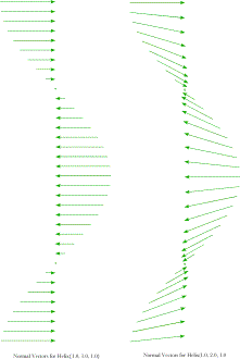
The normal vectors for two helices ( H{1.0,1.0 1.0} and H {1.0, 2.0, 1.0}) as viewed from the 90° direction.

In the above figure, the green vectors are normal vectors of the indicated helices. Since normal vectors are at a right angles to the turning vectors and the tangent vectors, they point into the center of the helix. For the helix (1.0, 1.0, 1.0} (the left panel), the normal vector points centrally and horizontally. The center of rotation is in that direction, a distance equal to the square root of the scalar of the turning quaternion. In this instance, the distance is the square root of two, which means that the center of rotation is beyond the central axis. When the horizontal projection of the helix is elliptical, the normal vectors tend to point slightly up or down relative to their points of origin.

The normal vectors point in the direction of the radii of curvature. In the next figure the length of each radius of curvature is multiplied times the normal vector for each sampled value of . The helix is one that has an elliptical projection into the horizontal plane, Helix {1.0, 2.0, 1.0}. It is viewed from the side (left panel) and from above (right panel) to give a better impression of the distribution of the radii of curvature. The tips of the vectors trace the evolute of the helix.

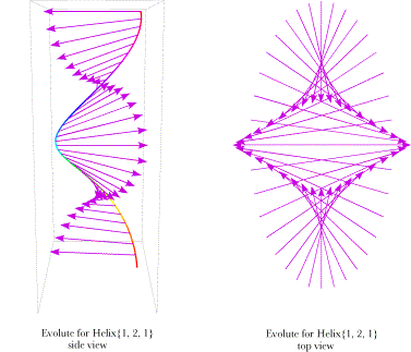
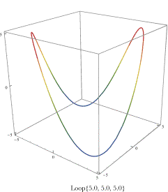
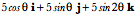
Distributions of the radii of curvature for the helix {1.0, 2.0, 1.0}. The radii are plotted as they would appear from the side (left panel) and from above (right panel). The tips of the arrows indicate the evolute of the helix.

The view from above is much like the evolute of an ellipse in the horizontal plane, but the evolute of an ellipse with the same shape is a smaller and more blunt ellipse. From the side view, it is apparent that the evolute of the helix is rather like a helix itself. Also note that the radii of curvature have a tendency to ascend or descend relative to their points of origin, which was true of the normal vectors for elliptical helices.

Another example of frames for a line in three-dimensional space

As a last example of framing of a line in three-dimensional space consider a closed line that will be called a loop. The formula for the vector that traces out the loop is similar to that for a helix except the k component is periodic.

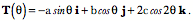
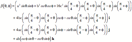
The closed loop is given by the above formula . It is a simple Lissajous figure in which the location vector is periodic in all three components.

The line is curved in all three directions, so it has a bit more complex frame. The tangent vectors, turning quaternion, and normal vectors are computed as they were for a helix.

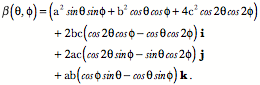
This expression for the turning vector, , causes some problems with calculation, therefore it can be rewritten in terms of and alone.

The unit normal vectors are obtained by rotating the unit tangent vector through 90° about the turning vector.

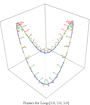
Frames for the loop {5.0, 5.0, 5.0} plotted at 10° intervals . The blue vectors are tangent vectors, the red vector turning vectors and the green vectors normal vectors. The loop is curved in all three directions. The loop is symmetrical about two vertical planes through opposite apices of the loop.

If the frames for the loop are calculated at 10° intervals then they appear as illustrated in the above figure. The frames are reasonable to casual inspection and they show the same symmetries as the loop itself. There are two planes of symmetry, both of them vertical and through opposite apices of the loop. The normal vectors near an apex are nearly in the plane of the curve and, as one move between apices, they twist smoothly through the intermediate directions.