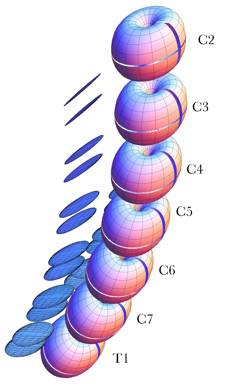
Spinal Dynamics III: Computing Compound Movements

When movements occur in the joints between bones, the configuration of the bones may change in complex ways. The overall changes may be simpler or more complex than the component movements. Consider an example. Your arm starts with the palm of your hand resting upon the anterior surface of your shoulder and you reach for a point directly in front of your shoulder. The trajectory of your hand is generally fairly simple, almost a straight line from your shoulder to the point. However, the component movements in your shoulder girdle, shoulder, elbow, wrist, and hand are all complex curvilinear movements. Conversely, consider a movement in the glenohumeral joint of your shoulder in which your arm swings into flexion from hanging straight down to above your head, about a fixed axis through the center of the humeral head and anatomical neck of the humerus. The movement is simple in the sense that it may be described by a single simple expression. However, the trajectory that is traced is fairly complex and not easily described without equations or actually performing the movement. The trajectory was computed and plotted at the end of Chapter 3.

In the lower cervical spine, we have a complex configuration of bones that move in subtle ways, even when we simplify the situation and use a set of identical elements with only two allowed types of movements between pairs of bones in the chain. The movements of the lower cervical spine may follow elegant arcs, as when a ballerina moves, but it is difficult to describe those movements precisely in words. At this section, we will try to capture something of the nature of such movements. Still, the discussion will be sketchy, both because this type of analysis is just beginning to be undertaken and because the movements are complex.

How can one characterize the movements, where the component movements are circular arcs in individual joints, but the concatenations of these simple movements are generally curvilinear but generally not circular arcs? If we return to the example of reaching from one’s shoulder to a point in space, the movement is simplified by noticing that the hand is essentially translated and rotated. Translation moves the hand from one location to another without changing its orientation and rotation turns it to be appropriately oriented. Such a movement will be called a compound movement. In this case, the equivalent compound movement is much simpler than the actual movement or its component movements, but that equivalent movement describes the overall functional structure of the movement. It clearly does not fully characterize the movement, not even the movement of the hand. As was pointed out in chapter 1, there are thirty-some possible degrees of freedom in the joints responsible for the movement and the equivalent compound movement has a maximum of six degrees of freedom. There is a great deal of internal structure arising from the anatomy of the joints and the temporal and functional linkages between the movements in the joints.

Similar constraints apply in the lower cervical spine, even in a simple model of that structure. In this discussion we will attempt only a very simple analysis of its movements.

First, consider the lower cervical spine in neutral position. The six cervical vertebrae will be considered to be identical in the relevant components of the vertebral body, the articular pillar, and the intervertebral discs.

The vertebral body is visually represented by a fat torus that is of the same relative height, width, and depth as a standard vertebral body (depth : height : width :: 0.8 : 1.0 : 1.4). The torus has been sliced horizontally and vertically so that the intersection of the cuts occurs in the anterior midline of the vertebral body. Those cuts are meant to visually indicate the orientation of the vertebral body.

.

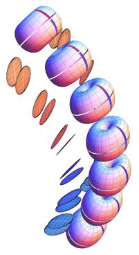
The artificial necks analyzed in this chapter begin in a neutral configuration like that illustrated by this visual model. The bodies are represented by flattened fat tori and the facet joints by flat discs. Intervertebral discs are indicted by the spacing between the tori. The actual computational model is a set of framed vectors and the rules that link them together.

The discs are indicated by a space between the vertebrae that is one half the height of a vertebral body. The facet joints are represented by two discs on each side, one for the superior facet and one for the inferior facet. Those discs are of the correct size shape and inclination for the standard facets of the lower cervical vertebrae. They are placed so that they are appropriately aligned and spaced to correspond with the alignment and spacing of the facets in actual cervical spines.

The rest of the features of the cervical vertebrae will be ignored for present purposes. The anatomy of the lower cervical spine has been measured in some detail and it is described elsewhere, as the basis for the model used here (Langer 2005q; Langer 2005r; Langer 2005s)

The vertebral bodies are tilted 6° relative to each other and they rest upon the T1 vertebra, which is tilted 30° anterior to the coronal plane. These parameters give a gently curved artificial neck that compares well with the average configuration of a number of necks imaged in x-rays, MRI, and serial sections of the neck.

The actual computational model is a set of framed vectors that include the location and orientation of the vertebral bodies, the facet joints, and the axes of rotation for movements in the sagittal plane and movements about an oblique axis. Rules are given for the concatenation of the vertebrae, so that movements of one vertebra are appropriately transmitted though the chain to all the connected vertebrae. The configuration of the lower cervical spine in neutral position is specified at the outset of a calculation, along with the movements that will occur in each joint. The consequences of a straight spine and a number of differently tilted spines are explored to some extent elsewhere (Langer 2005s). Rotational excursions about transverse axes and oblique axes are specified for each intervertebral joint and the resulting configuration of the spine is computed. The details of the model are given elsewhere (Langer 2005r).

As an example of the application of the model, consider the neck when the movements in each joint are into extension. In actual necks, it appears that the greatest excursions typically occur in the joints to either side of the C5 vertebra (C4/C5 and C5/C6), less in the adjacent joints (C3/C4 and C6/C7) and least in the joints between the extreme vertebrae at each end of the chain (C2/C3 and C7/T1). Measurements published in a number of sources would suggest that if the excursions are 5°, 7.5°, 10°, 10°, 7.5°, and 5° respectively, then the configuration should be a reasonable approximation to full extension in an actual neck. That configuration is illustrated in the following figure. It yields an overall movement of the C2 vertebra consistent with published figures (Kapandji 1974; Hoppenfeld 1976; Johnson, Hart et al. 1977; White and Panjabi 1978; Dvorak, Penning et al. 1988; Nordin and Frankel 1989; Panjabi and White 1989; Penning 1989; White and Panjabi 1990; Milne 1991; Committee 1998; Ghanayem, Zdeblick et al. 1998; Onan, Heggeness et al. 1998; Panjabi, Dvorak et al. 1998; Bogduk 1999; Bogduk and Mercer 2000; Levangie and Norkin 2001).

There is considerable variation from source to source in the magnitudes of the movements between the vertebrae and of the cervical spine in toto and there is substantial variation from neck to neck in the anatomical details of the vertebrae (Langer 2005q). Consequently, it would be a mistake to become wedded to any particular numbers for the angular excursions between cervical vertebrae. The combination chosen here gives a symmetrical anatomy that is reasonably consistent with published data and an image that is a good match to actual necks in full extension, therefore we will use it for the present discussion. One of the advantages of having a model such as this is that it is easy to plug in a series of scenarios and see how much difference they make to the final outcome. A fairly wide variety of joint excursions give much the same qualitative result, indicating that one has reasonable room for choice.

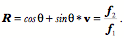
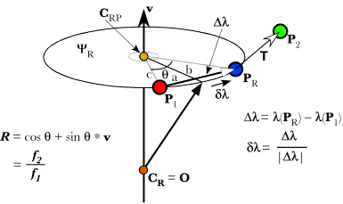
Drawing of a lower cervical spine in full extension assuming typical movements in each joint.

Compound movements in the cervical spine

One of the characteristics that strikes one immediately when studying such artificial spines is that the excursions of the upper vertebrae are much greater than those of the lower vertebrae. Obviously that is because movements of the more caudal vertebrae move more rostral vertebrae. As a result, the C2 vertebra moves through 45° of extension when the neck moves into full extension as modeled above. It also moves a considerable distance dorsally and some distance caudally. Let us now consider the movements in a more quantitative way. To start, we need to develop the methodology for measuring compound movements.

For each vertebra we know its location and orientation in neutral position and in full extension. Therefore, we can ask to what extent the movements are a pure swing in the sagittal plane. To determine to what extent the movement is a pure swing we need to compute the center of rotation for a planar movement, . What we know is the initial placement, , and the final placement, , and a point of reference, , which will the origin of the local coordinate system. As a first step, we can ask what rotation, , will carry the orientation of the vertebra in neutral position, , into the orientation in full extension, . R is the ratio of the frame of reference for the extended vertebra to the frame of reference for the vertebra in neutral position. The scalar of codes the angular excursion, .

We then compute the consequences of rotating the location of the initial placement, , by the same quaternion. The result is a new location, , that is usually different from the location of the second placement, .

Note that all these locations are defined relative to a center of rotation, , that is taken to be the local origin of the coordinate system. That turns out to be important, because the location of determines the form of the compound movement.

If is different from , then there is a translation, T, that carries into .

Translation does not change orientation, so we know that the orientation of the computed placement, , is the same as that for the final placement, .

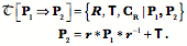
The placement is transformed into the placement by a combination of a rotation and a translation . The conical rotation about can be replaced by the pure swing about the center or rotation .

We now have the defining elements for the transformation of into .

With this information, it is possible to compute the center of rotation for the pure swing, , that will rotate into . We start with the observation that the axis of rotation is the unit vector of the rotation, .

Since is the local origin for conical rotations, the locations and are expressed in terms of it. Note that if is coincident with , then will also be coincident and the compound movement will be a rotation in place and a translation from to . However, is seldom coincident with any of the placement locations, therefore, we expect there to be a center of rotation for a pure swing that is not coincident with either placement. It is important to note that the choice of the center of rotation origin determines the locations of the swing centers. In words, the form of the compound movement is a function of the context in which it is seen to be occurring.

To find the center of rotation, , one can start by noticing that it lies in the plane of the rotation quaternion, on the perpendicular bisector of the line that connects the locations of and , and that the angle between the two locations is the angle of the rotation quaternion, . The vector that connects the two locations is .

The unit vector in the direction of is .

The location of the intersection between the perpendicular bisector and the line connecting the locations is .

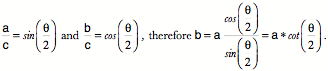
The bisector, the first half of the line connecting the locations, and the line that connects the center of rotation to the first location form a right triangle. The lengths of the sides of that triangle will be denoted by b, c, and a, respectively. Clearly, the length a is half the distance between the locations.

The angle at the apex of the triangle at the center of rotation is , therefore the following relations hold.

The vector pointing along the perpendicular bisector towards the center of rotation is the vector of the quaternion of the ratio of the axis of rotation to the vector between the locations. However, because the vector between the locations lies in the plane of the axis of rotation, the ratio quaternion is a vector .

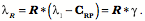
Now we can write down the location of the center of rotation for a pure swing movement that rotates into .

If we denote the vector from to as , then we can write the expression for the pure swing.

Bogduk, N. (1999). "The neck." Baillieres Best Pract Res Clin Rheumatol 13(2): 261-285.

Bogduk, N. and S. Mercer (2000). "Biomechanics of the cervical spine. I: Normal kinematics." Clin Biomech (Bristol, Avon) 15(9): 633-48.

Committee, T. C. S. R. S. E. (1998). The Cervical Spine. Phiadelphia, Lippincott - Raven.

Dvorak, J., L. Penning, et al. (1988). "Functional diagnostics of the cervical spine using computer tomography." Neuroradiology 30: 132-137.

Ghanayem, A. J., T. A. Zdeblick, et al. (1998). Functional Anatomy of Joints, Ligaments, and Discs. The Cervical Spine. T. C. S. R. S. E. Committee. Philidelphia, Lippincott - Raven: 45 - 52.

Hoppenfeld, S. (1976). Physical Examination of the Spine and Extremities. New York, Appleton-Century-Crofts.

Johnson, R. M., D. L. Hart, et al. (1977). "Cervical orthoses:a study comparing their effectiveness in restricting cervical motion in normal subjects." J Bone Jt Surg 59A: 332-339.

Kapandji, I. A. (1974). The Physiology of the Joints. Annotated diagrams of the mechanics of the human joints. New York, Churchill Livingstone.

Langer, T. P. (2005q). Building a Neck and Watching It Move: Anatomical Foundations for the Description of Movements in the Cervical Spine.: http://homepage.mac.com/tlanger_sasktel_net/CervicalSpine/lowercervical.html.

Langer, T. P. (2005r). A Model for the Study of Movements of the Lower Cervical Spine. : http://homepage.mac.com/tlanger_sasktel_net/CervicalSpine/lowercervical.html.

Langer, T. P. (2005s). Movements in Artificial Necks.: http://homepage.mac.com/tlanger_sasktel_net/CervicalSpine/lowercervical.html.

Levangie, P. K. and C. C. Norkin (2001). Joint Structure and Function. A Comphrehensive Analysis. Philadelphia, F. A. Davis Company.

Milne, N. (1991). "The role of zagapophyseal joint orientation and uncinate processes in controlling motion in the cervical spine." J. Anat. 178: 189.

Nordin, M. and V. H. Frankel (1989). Basic Biomechanics of the Musculoskeletal System. Philadelphia, Lea & Febiger.

Onan, O. A., M. H. Heggeness, et al. (1998). "A motion analysis of the cervical facet joint." Spine 23(4): 430-9.

Panjabi, M. M., J. Dvorak, et al. (1998). Cervical Spine Kinematics and Clinical Instability. The Cervical Spine. T. C. S. R. S. E. Committee. Philadelpia, Lippincott - Raven: 53 - 78.

Panjabi, M. M. and A. A. White (1989). Biomechanics of Nonacute Cervical Spinal Cord Injuries. The Cervical Spine. T. C. S. R. S. E. Committee. Philadelphia, J.B Lippincott: 91 - 96.

Penning, L. (1989). Functional Anatomy of Joints and Discs. The Cervical Spine. T. C. S. R. S. E. Committee. Philadelphia, J.B. Lippincott: 33 - 56.

White, A. A. and M. M. Panjabi (1978). Clinical Biomechanics of the Spine. Philadelphia, J. B. Lippincott.

White, A. A. and M. M. Panjabi (1990). Clinical Biomechanics of the Spine. Philadelphia, J.B. Lippincott.